petitRADTRANS Interface
You can find this notebook (and data) on GitHub. We demonstrate the use of gcm_toolkit with petitRADTRANS on a set of data of HD209458b simulations from Schneider et al. (2022).
Phase Curve
NOTE: phasecurves require petitRADTRANS AND prt_phasecure
Lets start with getting some gcmdata:
[1]:
import matplotlib.pyplot as plt
from gcm_toolkit import GCMT
import numpy as np
from petitRADTRANS import Radtrans
import astropy.constants as const
import astropy.units as u
Lets start with getting some gcmdata:
[2]:
!wget -O HD2.tar.gz https://figshare.com/ndownloader/files/36234516
!tar -xf HD2.tar.gz
--2022-08-23 08:49:13--  https://figshare.com/ndownloader/files/36234516
Resolving figshare.com (figshare.com)... 52.30.212.171, 34.250.160.50
Connecting to figshare.com (figshare.com)|52.30.212.171|:443... connected.
HTTP request sent, awaiting response... 302 Found
Location: https://s3-eu-west-1.amazonaws.com/pfigshare-u-files/36234516/HD2.tar.gz?X-Amz-Algorithm=AWS4-HMAC-SHA256&X-Amz-Credential=AKIAIYCQYOYV5JSSROOA/20220823/eu-west-1/s3/aws4_request&X-Amz-Date=20220823T064913Z&X-Amz-Expires=10&X-Amz-SignedHeaders=host&X-Amz-Signature=21232a3389137bcdbb4c7c0cf4fa1f27b58aeb1e4078b60f27c26b9453b552e4 [following]
--2022-08-23 08:49:13--  https://s3-eu-west-1.amazonaws.com/pfigshare-u-files/36234516/HD2.tar.gz?X-Amz-Algorithm=AWS4-HMAC-SHA256&X-Amz-Credential=AKIAIYCQYOYV5JSSROOA/20220823/eu-west-1/s3/aws4_request&X-Amz-Date=20220823T064913Z&X-Amz-Expires=10&X-Amz-SignedHeaders=host&X-Amz-Signature=21232a3389137bcdbb4c7c0cf4fa1f27b58aeb1e4078b60f27c26b9453b552e4
Resolving s3-eu-west-1.amazonaws.com (s3-eu-west-1.amazonaws.com)... 52.92.0.88
Connecting to s3-eu-west-1.amazonaws.com (s3-eu-west-1.amazonaws.com)|52.92.0.88|:443... connected.
HTTP request sent, awaiting response... 200 OK
Length: 18459732 (18M) [application/gzip]
Saving to: ‘HD2.tar.gz’

HD2.tar.gz          100%[===================>]  17.60M  14.5MB/s    in 1.2s

2022-08-23 08:49:15 (14.5 MB/s) - ‘HD2.tar.gz’ saved [18459732/18459732]
When loading the data, we make sure to use a low resolution of 15 degrees, since we need to calculate a lot of individual spectra.
[3]:
data = 'HD2_test/run'   # path to data
tools = GCMT(p_unit='bar', time_unit='day')  # create a GCMT object
tools.read_raw('MITgcm', data, iters="all", prefix=['T','U','V','W'], tag='HD2', d_lat=15, d_lon=15)
================================================================================
                             Welcome to gcm_toolkit
================================================================================
[STAT] Set up gcm_toolkit
   [INFO] pressure units: bar
   [INFO] time units: day
[STAT] Read in raw MITgcm data
   [INFO] File path: HD2_test/run
   [INFO] Iterations: 38016000, 41472000
time needed to build regridder: 0.34761476516723633
Regridder will use conservative method
   [INFO] Tag: HD2
Lets make sure we setup petitRADTRANS to get going. We will do the calculation only in the IR range where spitzer is located. You can of cause do the phase curve also for a broader wavelengthcoverage, or with exo-k low resolution opacities.
[4]:
pRT = Radtrans(line_species=['H2O_Exomol', 'Na_allard', 'K_allard', 'CO2', 'CH4', 'NH3', 'CO_all_iso_Chubb', 'H2S', 'HCN', 'SiO', 'PH3', 'TiO_all_Exomol', 'VO', 'FeH'],
               rayleigh_species=['H2', 'He'],
               continuum_opacities=['H2-H2', 'H2-He', 'H-'],
               wlen_bords_micron=[3.5, 4.6],
               do_scat_emis=True)
# Note: the pRT.setup_opa_structure is done by tools internally
Emission scattering is enabled: enforcing test_ck_shuffle_comp = True
  Read line opacities of H2O_Exomol...
 Done.
  Read line opacities of Na_allard...
 Done.
  Read line opacities of K_allard...
 Done.
  Read line opacities of CO2...
 Done.
  Read line opacities of CH4...
 Done.
  Read line opacities of NH3...
 Done.
  Read line opacities of CO_all_iso_Chubb...
 Done.
  Read line opacities of H2S...
 Done.
  Read line opacities of HCN...
 Done.
  Read line opacities of SiO...
 Done.
  Read line opacities of PH3...
 Done.
  Read line opacities of TiO_all_Exomol...
 Done.
  Read line opacities of VO...
 Done.
  Read line opacities of FeH...
 Done.

  Read CIA opacities for H2-H2...
  Read CIA opacities for H2-He...
Done.
Set some arguments for petitradtrans. Check the docs to see what arguments need to be set. The gravity can be obtained from the GCMT dataset.
[6]:
MMW = const.R.si.value / 3590 * 1000
Rstar = 1.203*const.R_sun.cgs.value
Tstar = 6092.0
semimajoraxis = (0.04747 * u.au).cgs.value
Set the phases (from 0 to 1 is a full phasecurve, where 0.5 is the nightside and 0.0=1.0 is the dayside) for which you want to integrate the spectra.
We also need to create the interface object
[7]:
phases = np.linspace(0,1,50)
interface = tools.get_prt_interface(pRT)
Lets link the gcm data to the interface. At this point we also need to decide at which timestep we want to do the calculation. We decide here to use the latest.
[8]:
interface.set_data(time=12000, tag='HD2')
We can now decide on the chemistry that we want to use. We currently only support pRTs poorman chemistry.
[9]:
interface.chem_from_poorman('T', co_ratio=0.55, feh_ratio=0.0) # the temperature key sets the gcm key used for the temperature
We can now calculate the spectrum and save it to a file. This step will take some time, depending on the resolution that you chose.
[10]:
filename = 'spectrum.nc'
interface.calc_phase_spectrum(mmw=MMW, filename=filename, Rstar=Rstar, Tstar=Tstar, semimajoraxis=semimajoraxis, normalize=True);
100%|█████████████████████████████████████████| 288/288 [09:34<00:00, 1.99s/it]
The final planet to star flux ratio needs to be accounted for the planetary and stellar radii (see e.g., Sing et al. 2018, eq.2)
\(\frac{\Delta f}{f} = \left(\frac{R_\mathrm{pla}}{R_\mathrm{star}}\right)^2 \frac{F_\mathrm{pla}}{F_\mathrm{star}}\)
interface.calc_phase_spectrum does this automatically for you. Set normalize=False, if you prefer the uncorrected spectrum.
[11]:
ph = interface.phase_curve(phases,filename=filename)require
Lets do some nice plots. Lets start with the emission spectra:
[12]:
# Dayside = phase == 0
(ph*1e6).sel(phase=0).plot()
plt.xscale('log')
plt.yscale('linear')
plt.xlim([3.5,4.6])
plt.ylim([500,3000])
plt.ylabel(r'$F_\mathrm{pl}/F_\mathrm{star}$ [ppm]')
plt.xlabel('$\lambda$ [$\mu$m]')
plt.title('Dayside emission spectrum')
plt.show()

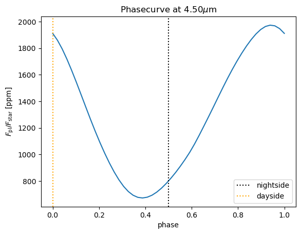
Here are some phasecurves in the spitzer wavelengths:
[13]:
# 4.5 mu m plot
l = 4.5
(ph*1e6).interp(wlen=l).plot()
plt.axvline(0.5, label='nightside', ls=':', color='black')
plt.axvline(0.0, label='dayside', ls=':', color='orange')
plt.xlabel('phase')
plt.ylabel(r'$F_\mathrm{pl}/F_\mathrm{star}$ [ppm]')
plt.title(r'Phasecurve at {:.2f}$\mu$m'.format(l))
plt.legend()
plt.show()
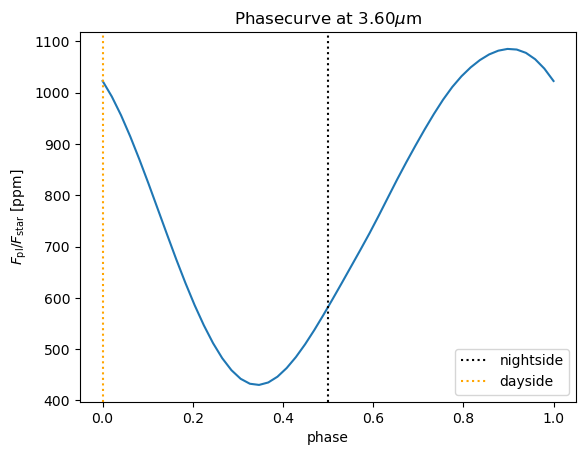
# 3.6 mu m plot
l = 3.6
(ph*1e6).interp(wlen=l).plot()
plt.axvline(0.5, label='nightside', ls=':', color='black')
plt.axvline(0.0, label='dayside', ls=':', color='orange')
plt.xlabel('phase')
plt.ylabel(r'$F_\mathrm{pl}/F_\mathrm{star}$ [ppm]')
plt.title(r'Phasecurve at {:.2f}$\mu$m'.format(l))
plt.legend()
plt.show()
Transit Spectrum
Next we show how to calculate a transmission spectrum using the petitRADTRANS interface of gcm_toolkit. We use the same data as for the phase curve and start by setting up gcm_toolkit and petitRADTRANS:
[7]:
# get data
!wget -O HD2.tar.gz https://figshare.com/ndownloader/files/36234516
!tar -xf HD2.tar.gz

# initialise gcm_tookit
data = 'HD2_test/run'   # path to data
tools = GCMT(p_unit='bar', time_unit='day')  # create a GCMT object
tools.read_raw('MITgcm', data, iters="all", prefix=['T','U','V','W'], tag='HD2', d_lat=1, d_lon=1)

# initialise petitRADTRANS
pRT = Radtrans(line_species=['H2O_Exomol', 'Na_allard', 'K_allard', 'CO2', 'CH4', 'NH3', 'CO_all_iso_Chubb', 'H2S', 'HCN', 'SiO', 'PH3', 'TiO_all_Exomol', 'VO', 'FeH'],
               rayleigh_species=['H2', 'He'],
               continuum_opacities=['H2-H2', 'H2-He', 'H-'],
               wlen_bords_micron=[0.3, 10])

# connect petitRADTRANS and gcm_toolkit
interface = tools.get_prt_interface(pRT)
--2023-02-27 06:45:38--  https://figshare.com/ndownloader/files/36234516
Resolving figshare.com (figshare.com)... 34.252.222.205, 54.217.34.18, 2a05:d018:1f4:d000:647c:7301:fad1:b2b9, ...
Connecting to figshare.com (figshare.com)|34.252.222.205|:443... connected.
HTTP request sent, awaiting response... 302 Found
Location: https://s3-eu-west-1.amazonaws.com/pfigshare-u-files/36234516/HD2.tar.gz?X-Amz-Algorithm=AWS4-HMAC-SHA256&X-Amz-Credential=AKIAIYCQYOYV5JSSROOA/20230227/eu-west-1/s3/aws4_request&X-Amz-Date=20230227T054538Z&X-Amz-Expires=10&X-Amz-SignedHeaders=host&X-Amz-Signature=f3173652eeecb44749cd6f18cb6c495b531eb4216ce94dfcc78c32d0155e5df1 [following]
--2023-02-27 06:45:38--  https://s3-eu-west-1.amazonaws.com/pfigshare-u-files/36234516/HD2.tar.gz?X-Amz-Algorithm=AWS4-HMAC-SHA256&X-Amz-Credential=AKIAIYCQYOYV5JSSROOA/20230227/eu-west-1/s3/aws4_request&X-Amz-Date=20230227T054538Z&X-Amz-Expires=10&X-Amz-SignedHeaders=host&X-Amz-Signature=f3173652eeecb44749cd6f18cb6c495b531eb4216ce94dfcc78c32d0155e5df1
Resolving s3-eu-west-1.amazonaws.com (s3-eu-west-1.amazonaws.com)... 52.218.29.83, 52.218.120.72, 52.218.36.82, ...
Connecting to s3-eu-west-1.amazonaws.com (s3-eu-west-1.amazonaws.com)|52.218.29.83|:443... connected.
HTTP request sent, awaiting response... 200 OK
Length: 18459732 (18M) [application/gzip]
Saving to: ‘HD2.tar.gz’

HD2.tar.gz          100%[===================>]  17.60M  2.34MB/s    in 5.7s

2023-02-27 06:45:44 (3.10 MB/s) - ‘HD2.tar.gz’ saved [18459732/18459732]

tar: Ignoring unknown extended header keyword 'LIBARCHIVE.xattr.com.apple.metadata:_kMDItemUserTags'
tar: Ignoring unknown extended header keyword 'LIBARCHIVE.xattr.com.apple.FinderInfo'
tar: Ignoring unknown extended header keyword 'LIBARCHIVE.xattr.com.apple.metadata:_kMDItemUserTags'
tar: Ignoring unknown extended header keyword 'LIBARCHIVE.xattr.com.apple.metadata:_kMDItemUserTags'
tar: Ignoring unknown extended header keyword 'LIBARCHIVE.xattr.com.apple.metadata:_kMDItemUserTags'
tar: Ignoring unknown extended header keyword 'LIBARCHIVE.xattr.com.apple.metadata:_kMDItemUserTags'
tar: Ignoring unknown extended header keyword 'LIBARCHIVE.xattr.com.apple.lastuseddate#PS'
tar: Ignoring unknown extended header keyword 'LIBARCHIVE.xattr.com.apple.FinderInfo'
tar: Ignoring unknown extended header keyword 'SCHILY.fflags'
tar: Ignoring unknown extended header keyword 'LIBARCHIVE.xattr.com.apple.metadata:_kMDItemUserTags'
tar: Ignoring unknown extended header keyword 'LIBARCHIVE.xattr.com.apple.metadata:_kMDItemUserTags'
tar: Ignoring unknown extended header keyword 'SCHILY.fflags'
================================================================================
                             Welcome to gcm_toolkit
================================================================================
[STAT] Set up gcm_toolkit
   [INFO] pressure units: bar
   [INFO] time units: day
[STAT] Read in raw MITgcm data
   [INFO] File path: HD2_test/run
   [INFO] Iterations: 41472000, 38016000
time needed to build regridder: 2.923800468444824
Regridder will use conservative method
   [INFO] Tag: HD2
  Read line opacities of H2O_Exomol...
 Done.
  Read line opacities of Na_allard...
 Done.
  Read line opacities of K_allard...
 Done.
  Read line opacities of CO2...
 Done.
  Read line opacities of CH4...
 Done.
  Read line opacities of NH3...
 Done.
  Read line opacities of CO_all_iso_Chubb...
 Done.
  Read line opacities of H2S...
 Done.
  Read line opacities of HCN...
 Done.
  Read line opacities of SiO...
 Done.
  Read line opacities of PH3...
 Done.
  Read line opacities of TiO_all_Exomol...
 Done.
  Read line opacities of VO...
 Done.
  Read line opacities of FeH...
 Done.

  Read CIA opacities for H2-H2...
  Read CIA opacities for H2-He...
 Done.
To calculate a transit spectrum, the data has to be prepared. For this, we use the set_data function by setting terminator_avg to True. Furthermore, we need to decide the longitudinal opening angle. This will define over which longitudinal angle around the terminators the temperature will be averaged. Furthermore, we need to set the number of latitudinal points per terminator. For each of this point, a transmission spectrum will be calculated and averaged for the final spectrum.
[8]:
interface.set_data(time=12000, tag='HD2', terminator_avg=True, lat_points=1, lon_resolution=10)
Next, the chemistry needs to be calculated. This again is the same as for the phase curve.
[9]:
interface.chem_from_poorman('T', co_ratio=0.55, feh_ratio=0.0)
After everything is set up, the transit spectrum can be calculated using the calc_transit_spoectrum function. The only remaining parameter that needs to be given is the mean molecular weight of the atmosphere.
Note: The wavelength is given in micron and the spectra is the planet radius in cm.
[10]:
wave, spectra = interface.calc_transit_spectrum(2.33)
<xarray.Dataset>
Dimensions:         (lon: 2, lat: 1, Z: 47)
Coordinates:
  * lon             (lon) int64 -90 90
  * lat             (lat) float64 0.0
  * Z               (Z) float64 650.0 550.0 450.0 ... 3.633e-05 2.471e-05 1e-05
Data variables: (12/23)
    T               (lon, lat, Z) float64 4e+03 4e+03 ... 1.227e+03 1.391e+03
    H2              (lon, lat, Z) float64 0.7128 0.7106 0.7078 ... 0.7381 0.7374
    He              (lon, lat, Z) float64 0.2495 0.2495 0.2495 ... 0.2495 0.2495
    CO              (lon, lat, Z) float64 0.004843 0.004976 ... 0.005521
    H2O             (lon, lat, Z) float64 0.003063 0.002967 ... 0.002459
    HCN             (lon, lat, Z) float64 7.453e-05 6.743e-05 ... 2.196e-12
    ...              ...
    e-              (lon, lat, Z) float64 1.339e-10 1.448e-10 ... 1.546e-12
    H-              (lon, lat, Z) float64 5.911e-08 5.861e-08 ... 2.002e-16
    H               (lon, lat, Z) float64 0.02501 0.02719 ... 0.0005425
    FeH             (lon, lat, Z) float64 0.0001677 0.0001554 ... 2.58e-09
    MMW             (lon, lat, Z) float64 2.266 2.261 2.253 ... 2.331 2.324 2.33
    nabla_ad        (lon, lat, Z) float64 0.1711 0.1682 0.1647 ... 0.2765 0.246
Attributes:
    p_unit:   bar
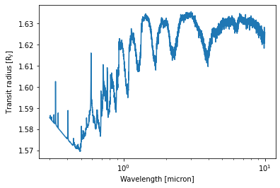
The final transmission spectrum is shown below. We divided by the radius of Jupiter to give the transit depth in Jupiter radii.
[12]:
plt.figure()
plt.plot(wave, spectra/6991100000)
plt.xscale('log')
plt.xlabel('Wavelength [micron]')
plt.ylabel('Transit radius [R$_J$]')
plt.show()