Getting started
You can find this notebook (and data) on GitHub. We demonstrate the use of gcm_toolkit on a set of data of HD209458b simulations from Schneider et al. (2022).
Lets start with getting some testdata:
!wget -O HD2.tar.gz https://figshare.com/ndownloader/files/36234516 !tar -xf HD2.tar.gz
import all needed packages
[1]:
import matplotlib.pyplot as plt
from gcm_toolkit import GCMT
from gcm_toolkit import gcm_plotting as gcmp
This tutorial will showcase how to use the GCMT package to load and analyze MITgcm data (raw binary format). Lets take a look at how easy it is to load data from a MITgcm run.
[2]:
data = 'HD2_test/run'   # path to data
tools = GCMT(p_unit='bar', time_unit='day')  # create a GCMT object
tools.read_raw('MITgcm', data, iters="all", prefix=['T','U','V','W'], tag='HD2')
================================================================================
                             Welcome to gcm_toolkit
================================================================================
[STAT] Set up gcm_toolkit
   [INFO] pressure units: bar
   [INFO] time units: day
[STAT] Read in raw MITgcm data
   [INFO] File path: HD2_test/run
   [INFO] Iterations: 38016000, 41472000
time needed to build regridder: 0.8844950199127197
Regridder will use conservative method
   [INFO] Tag: HD2
We can also retrieve an xarray dataset from the GCMT object, for further use.
[3]:
ds = tools['HD2']
# ds = tools.models # note this is equal, since we only loaded one dataset
Check the content of the dataset:
[4]:
# ds
Plot data
We now demonstrate how to do simple plots of the data. We start with an isobaric slice of the temperature.
Don’t forget to checkout the options for the plotting functions.
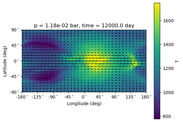
[5]:
tools.isobaric_slice(pres=1e-2, lookup_method='nearest', var_key='T', wind_kwargs={'windstream':False, 'sample_one_in':2})
[STAT] Plot Isobaric slices
   [INFO] Variable to be plotted: T
   [INFO] Pressure level: 0.01
[STAT] Plot horizontal winds
Note that tools wraps the plot functions defined in tools.gcm_plotting. You achieve the same with:
[6]:
gcmp.isobaric_slice(ds, pres=1e-2, lookup_method='nearest', var_key='T', wind_kwargs={'windstream':False, 'sample_one_in':2})
[STAT] Plot Isobaric slices
   [INFO] Variable to be plotted: T
   [INFO] Pressure level: 0.01
[STAT] Plot horizontal winds

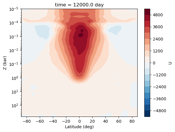
We can also do a zonal mean of the wind.
[7]:
tools.zonal_mean('U', contourf = True, levels =20)
[STAT] Plot zonal mean
   [INFO] Variable to be plotted: U
Advanced plotting with cartopy
Plots look a lot nicer, if we use cartopy. So lets do it.
[8]:
import cartopy.crs as ccrs
PROJECTION = ccrs.Robinson()
[9]:
time = -1
fig, axes = plt.subplots(2,2,subplot_kw={'projection':PROJECTION}, figsize=(12,8), constrained_layout=True)
for i,Z in enumerate([1e-3, 1e-1,1e-2,1]):
    axt = axes.flat[i]
    tools.isobaric_slice(var_key='T',
                        ax=axt, pres=Z, time=time, lookup_method ='nearest',
                        wind_kwargs={'transform':ccrs.PlateCarree(),'windstream':True, 'arrow_color':'w','sample_one_in':2},
                        transform=ccrs.PlateCarree(), cmap=plt.get_cmap('inferno'),
                        contourf=True, levels=20,
                        cbar_kwargs={'pad':.005})
[STAT] Plot Isobaric slices
   [INFO] Variable to be plotted: T
   [INFO] Pressure level: 0.001
[STAT] Plot horizontal winds
[STAT] Plot Isobaric slices
   [INFO] Variable to be plotted: T
   [INFO] Pressure level: 0.1
[STAT] Plot horizontal winds
[STAT] Plot Isobaric slices
   [INFO] Variable to be plotted: T
   [INFO] Pressure level: 0.01
[STAT] Plot horizontal winds
[STAT] Plot Isobaric slices
   [INFO] Variable to be plotted: T
   [INFO] Pressure level: 1
[STAT] Plot horizontal winds
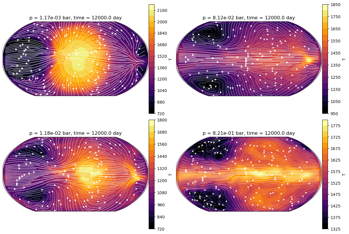
Using cartopy is very simple. Make sure to create an axes obeject with the keyword projection to set to a cartopy projection. You then use the transform keyword during plotting to set the coordinate system, that the data is defined in (ccrs.PlateCarree())
Postprocessing of data
Horizontal averages
We can do some additional post-processing, such as calculating global horizontal averages of the temperature
[10]:
tools.add_horizontal_average('T', 'T_g', tag='HD2');
[STAT] Calculate horizontal average
   [INFO] Output variable: T_g
   [INFO] Area of grid cells: area_c
   [INFO] Variable to be averaged: T
   [INFO] Performing global average
We can also calculate dayside, nightside, morning terminator or evening terminator averages or averages of quantities that are not part of the dataset. Here are some examples:
[11]:
tools.add_horizontal_average('T', 'T_evening', tag='HD2', part='evening');
tools.add_horizontal_average('T', 'T_morning', tag='HD2', part='morning');
tools.add_horizontal_average('T', 'T_night', tag='HD2', part='night');
tools.add_horizontal_average('T', 'T_day', tag='HD2', part='day');
tools.add_horizontal_average(ds.T, 'T_day', tag='HD2', part='day');  # is the same as above
[STAT] Calculate horizontal average
   [INFO] Output variable: T_evening
   [INFO] Area of grid cells: area_c
   [INFO] Variable to be averaged: T
   [INFO] Performing morning terminator average
[STAT] Calculate horizontal average
   [INFO] Output variable: T_morning
   [INFO] Area of grid cells: area_c
   [INFO] Variable to be averaged: T
   [INFO] Performing evening terminator average
[STAT] Calculate horizontal average
   [INFO] Output variable: T_night
   [INFO] Area of grid cells: area_c
   [INFO] Variable to be averaged: T
   [INFO] Performing nightside average
[STAT] Calculate horizontal average
   [INFO] Output variable: T_day
   [INFO] Area of grid cells: area_c
   [INFO] Variable to be averaged: T
   [INFO] Performing dayside average
[STAT] Calculate horizontal average
   [INFO] Output variable: T_day
   [INFO] Area of grid cells: area_c
   [INFO] Variable to be averaged is taken from input
   [INFO] Performing dayside average
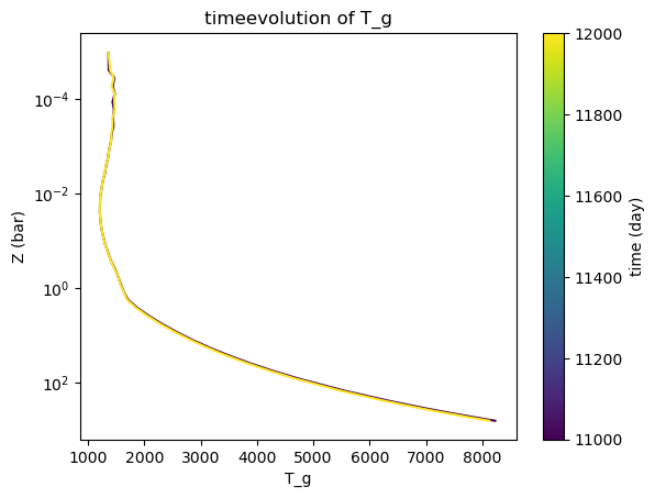
Lets think about the temperature evolution of the horizontally averaged temperature profile.
[12]:
tools.time_evol('T_g') # note that we only loaded two timesteps
[STAT] Plot horizontal winds
   [INFO] Variable to be plotted: T_g
[12]:
<matplotlib.collections.LineCollection at 0x17db80af0>
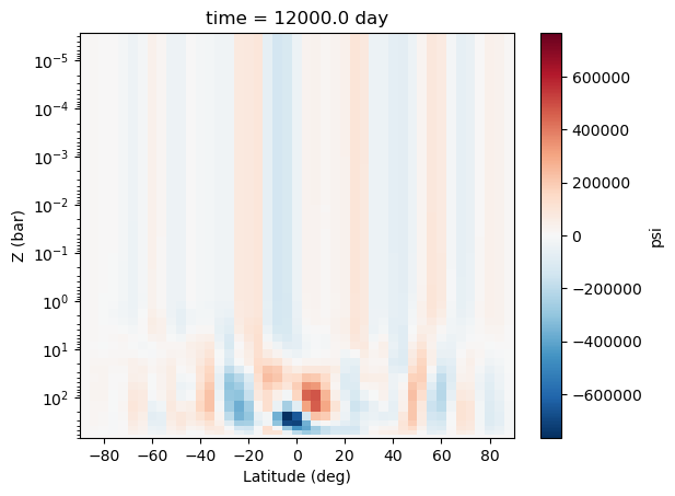
Meridional overturning circulation
Calculate overturning circulation
[13]:
tools.add_meridional_overturning(var_key_out='psi');
[STAT] Calculate meridional overturning streamfunction
   [INFO] Output variable: psi
[14]:
tools.zonal_mean('psi')
[STAT] Plot zonal mean
   [INFO] Variable to be plotted: psi
Total Energy
We can also calculate the total energy in the GCM
[15]:
tools.add_total_energy(var_key_out='E')
[STAT] Calculate total energy
   [INFO] Output variable: E
   [INFO] Area of grid cells: area_c
   [INFO] Temperature variable: T
[15]:
<xarray.DataArray (time: 2)>
array([1.00857669e+32, 9.96034924e+31])
Coordinates:
    iter     (time) int64 38016000 41472000
* time (time) float64 1.1e+04 1.2e+04Total Mementum
Or how about the total angular momentum?
[16]:
tools.add_total_momentum(var_key_out='TM')
[STAT] Calculate total angular momentum
   [INFO] Output variable: TM
   [INFO] Area of grid cells: area_c
   [INFO] Temperature variable: T
[16]:
<xarray.DataArray (time: 2)>
array([1.20453412e+35, 1.20551025e+35])
Coordinates:
    iter     (time) int64 38016000 41472000
* time (time) float64 1.1e+04 1.2e+04RCB
What if we want to know the location of the RCB? We can also do this
[17]:
tools.add_rcb(var_key_out='rcb')
[STAT] Calculate the location of the rcb
   [INFO] Output variable: rcb
   [INFO] Area of grid cells: area_c
   [INFO] Temperature variable: T
[STAT] Calculate horizontal average
   [INFO] Area of grid cells: area_c
   [INFO] Variable to be averaged: theta
   [INFO] Performing global average
[17]:
<xarray.DataArray 'Z' (time: 2)>
array([1.776412, 1.776412])
Coordinates:
    Z        (time) float64 1.776 1.776
    drF      (time) >f8 6.767e+04 6.767e+04
    PHrefC   (time) >f8 1.284e+08 1.284e+08
    iter     (time) int64 38016000 41472000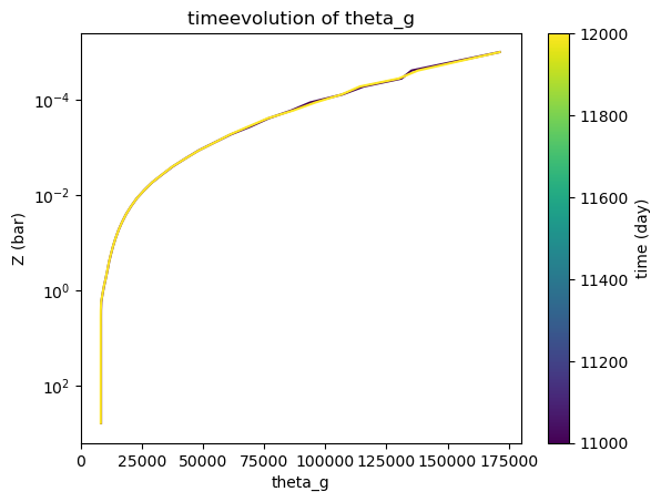
* time (time) float64 1.1e+04 1.2e+04Calculate potential temperature
We sometimes might be interested in the potential temperature as well, so we can calculate that as well.
[18]:
tools.add_theta('theta') # calculates theta
tools.add_horizontal_average('theta','theta_g')  # also calculate the global average
tools.time_evol('theta_g')  # note that we only loaded two timesteps
[STAT] Calculate horizontal average
   [INFO] Output variable: theta_g
   [INFO] Area of grid cells: area_c
   [INFO] Variable to be averaged: theta
   [INFO] Performing global average
[STAT] Plot horizontal winds
   [INFO] Variable to be plotted: theta_g
[18]:
<matplotlib.collections.LineCollection at 0x17c4573d0>
Dealing with the GCMT object
GCMT binds in naturally into the pythonic environment. Here are a few examples of how you can interact with the GCMT object:
print the amount of loaded models:
[19]:
len(tools)
[19]:
1
check if a model is loaded:
[20]:
bool(tools)
[20]:
True
iterate over models:
[21]:
for tag, ds in tools:
    print(tag, ds.Z.max().values)
HD2 650.0
Retrieve a model:
[22]:
ds = tools.get('HD2')   # pythonic get (you can also set a default)
ds = tools.get_models('HD2')  # GCMT get, with more options
ds = tools.get_one_model('HD2')  # can raise an error if you want to
ds = tools['HD2']  # normal pythonic __getitem__
Set a model:
[23]:
tools['HD2_clone'] = ds
You may want to check which of those is suited for your case. Just check the docs to find out:
[24]:
help(tools.get_models)
Help on method get_models in module gcm_toolkit.gcmtools:

get_models(tag=None, always_dict=False) method of gcm_toolkit.gcmtools.GCMT instance
    Function return all GCMs in memory. If a tag is given, only return this
    one.

    Parameters
    ----------
    tag : str
        Name of the model that should be returned.
    always_dict: bool
        Force result to be a dictionary (if tag is None)

    Returns
    -------
    selected_models : GCMDatasetCollection or xarray Dataset
        All models in self._models, or only the one with the right tag.
        Will definetly be GCMDatasetCollection if always_dict=True